COLD: Counterdiabatic Optimised Local Driving

Recently, my paper Counterdiabatic Optimised Local Driving (which I will refer to as COLD 🧊) finally got published in PRX Quantum!

I figured one of the best ways to communicate its results is to write a brief-ish blogpost focusing on 3 things:

Why you should care about speeding up adiabatic processes in quantum systems
How COLD is just the tool to do this (and what it actually does)
Why COLD is cool (ha)

This post turned out to be far longer than I’d anticipated but luckily it can also be read in bits and pieces in case you’re interested in certain aspects of eg adiabatic quantum computing, the variational approach to counterdiabatic driving and/or the adiabatic gauge potential. I’m hoping this is very accessible for anyone with a rudimentary knowledge of quantum mechanics, so please let me know if something gets too much!

Some time ago, I wrote a post explaining counterdiabatic driving (CD) for the IBM Quantum Aviary blog, a slightly different version of which also exists on this site. I don’t want to spend too long going over the same stuff so I recommend reading it if you’d like to get an easy and fun intro to the topic. I also recommend this thread for a speedier version:

What is Counterdiabatic Driving?

A thread for the Physicist, the Non-Physicist and every superposition of the above. I'll start with the simple and go progressively towards more quantum physics-y, but I hope this is interesting to most.

1/n
— ieva (@HyperboIeva) March 1, 2021

I’ll rehash the inner workings of CD in this post, but it will likely be a different and more involved perspective, so I recommend the links above to get an overview either before you dive deeper here or instead of it.

Adiabatic quantum computation

While I don’t think it’s necessary to understand adiabatic quantum processes solely from the point of view of quantum computation, it’s a nice and self-contained way of motivating and explaining the results of COLD so this is what I’ll start with (especially to those who come from less of an experimental/physics background – the experimentalists can already appreciate adiabaticity). The TLDR if you want to skip this section and get to the juicy bits concerning my paper is just:

Adiabatic Quantum Computation is simply the time-evolution of a Hamiltonian where the system is prepared in a particular initial state (eg ground state) and the Hamiltonian varies slowly in time such that it stays in that eigenstate.

The lengthy motivation as to why you should care about it proceeds from here on out.

First: adiabatic quantum computation (AQC) is known to be equivalent to circuit-based QC – up to a polynomial overhead which is at least theoretically efficient. Since the circuit model is universal for quantum computing, what I’m really trying to say is that you can do any computation you’d like using AQC. In practice, physicists (experimentalists) sometimes like to use AQC (or what one can simply refer to as adiabatic protocols) even more than the circuit model, since it translates more naturally to the quantum systems that they build and control. In fact, some quantum gates are implemented in their physical hardware using adiabatic protocols. Things like state preparation or algorithms for solving useful combinatorics problems are often more natural in the AQC setting.

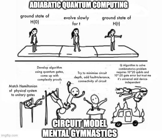
A (decently unfair but objectively funny) comparison of AQC and circuit-based QC.

The main difference between the two is that AQC relies on time-dependent Hamiltonian evolution rather than exploring the entire Hilbert space with a set of unitary quantum logic gates. In AQC (generally) the computation starts in an initial Hamiltonian whose ground state is easy to prepare and evolves to a final Hamiltonian whose ground state encodes the solution to the computational problem (see meme above). As for universality, a nice operational definition is that there is an efficient mapping of any circuit to an adiabatic computation given a sufficiently powerful Hamiltonian. In practice, Physicists often bypass the mapping part and just start straight from some physical system that encodes their problem already since that’s way easier.

I’ll stop here to note that I’m focusing on universality perhaps a bit too much – the true power of AQC is in solving very particular problems, not in adapting it to run an arbitrary quantum algorithm. I wanted to highlight the fact that there is a lot of space to explore wherein

For plenty of problems, this ‘useful’ physical system isn’t a very complicated one (see the power of the Ising Hamiltonian). One of the real issues in AQC is the condition of slow evolution (the other is a power requirement, but it’s a lot more nuanced so we’ll stick to slowness for now). For a process to be genuinely adiabatic in the quantum sense, it has to happen infinitely slowly. As mentioned in my other blog post, this is due to the quantum adiabatic theorem and exponentially small energy gaps of your system. So in practice, what we’re always dealing with are quasi-adiabatic processes, where a system gets driven slowly enough as to minimise these losses and transitions.

Importantly though, you can only go so slow. Notoriously, we’d like to compute things faster rather than slower and this holds even more true for quantum systems, where slow evolution allows for more decoherence and other unhelpful side effects.

This puts AQC between a rock and a hard place: go too fast and you get non-adiabatic transitions and losses, go too slow and you risk decoherence.

A slightly deeper dive into CD

The focus of our new method COLD is to find a way to speed up adiabatic processes while suppressing non-adiabatic losses. It is by no means the only one out there trying to accomplish this – there is an entire zoo of research papers focused on the topic, with many of them under the banner of shortcuts to adiabaticity (STA) (I recommend this review for anyone interested in finding out more). One key method in STA is counterdiabatic driving.

I want to take a different approach to my earlier blogpost and delve a little more into the physics of the counterdiabatic drive and this interesting thing called the adiabatic gauge potential. You can skip the rest of this section if you’re interested only in the bigger picture, but for anyone keen on getting an insight into how one derives the idea of a counterdiabatic drive, read on!

To start, let’s imagine a Hamiltonian $H(\lambda(t))$ acting on some system $|\psi \rangle$ which depends on time through the function $\lambda$ . You can always diagonalise it through some unitary transformation $U(\lambda(t))$ at each point in time, giving you a new, diagonal Hamiltonian:

$\Tilde{H}(\lambda) = U^{\dagger}(\lambda)H(\lambda)U(\lambda)$ .

Going to this “moving frame” also means transforming the wavefunction of the system:

$|\Tilde{\psi} \rangle = U(\lambda)|\psi \rangle$ .

If you then solve the Schrödinger eq. for this new wavefunction, what you find is that it evolves under a slightly different Hamiltonian than the one we defined above! In fact:

$i \hbar \frac{d |\Tilde{\psi}\rangle}{dt} = (\Tilde{H} - \dot{\lambda}\mathcal{A}_{\lambda})|\Tilde{\psi}\rangle$ ,

where the term $\mathcal{A}_{\lambda} = i\hbar U^{\dagger}\partial_{\lambda}U$ is the adiabatic gauge potential (AGP), a particularly fascinating object which can be seen as the generator of adiabatic transformations. The fact that it scales with the speed of your changing Hamiltonian (the $\dot{\lambda}$ term) means that the faster you go, the more non-adiabatic losses you should expect! I made a small, messy animation to show this:

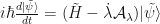
Time-dependent Hamiltonian in the moving frame basis for a slow (quasi-adiabatic) evolution and a fast one (non-adiabatic). The size of the blue spheres are the magnitudes of the entries of the diagonalised Hamiltonian and the red spheres are the non-adiabatic effects from the second term.

This is where counterdiabaticity start to come into the picture: say we know the AGP exactly for some problem Hamiltonian. We could essentially cancel out all those red spheres in the effective evolution Hamiltonian. In essence we’d just do exactly what you’d expect:

$H_{CD} = (\Tilde{H} - \dot{\lambda}\mathcal{A}_{\lambda}) + \dot{\lambda}\mathcal{A}_{\lambda} = \Tilde{H}$ ,

And voila! Your perfect Hamiltonian, driven arbitrarily quickly and yet never leaving the eigenstate it started in. The extra term is something you engineer and it exactly cancels out the non-adiabatic contributions. This is the counterdiabatic drive.

Given how simple the whole idea is and how useful adiabatic protocols are, the question then becomes: why don’t people do this all the time? I guess it’s unsurprising to find that the answer is “it’s harder than it looks”.

First, we find that the AGP satisfies a very specific relationship:

$\langle m| \mathcal{A} | n \rangle = i \hbar \langle m | \partial_{\lambda} n \rangle = -i\hbar \frac{\langle m| \partial_{\lambda} H | n \rangle}{E_m - E_n}$ ,

where $|n\rangle$ and $E_n$ are eigenstates and energies of the instantaneous Hamiltonian at each point in time. This tells you that it’s really complicated to derive. You’d need to know the full spectrum of your Hamiltonian at each instantaneous moment in time! Not only that, but engineering an arbitrary operator that looks like this is damn near impossible, especially when you get to big system sizes, no matter what quantum system you’re working with. Furthermore, once you get to exponentially small gaps between your eigenenergies (ie $|E_n - E_m| \ll 1$ ), the terms in the AGP blow up to infinity, meaning your experiment would need infinite power to produce these drives.

Basically, the exact CD is just about impossible to derive and/or implement in most scenarios, especially those that are interesting. So what can we do instead?

The variational approach

Many people have tried to tackle the complex problem of deriving and implementing the CD in the past. I won’t do a literature review, but it’s safe to say that it’s an open field of research. One recent approach, however, is more general and more practical than many and that is the approach we build upon in our new paper. We call it local counterdiabatic driving (LCD) and it was introduced in a paper by Sels and Polkovnikov in 2017.

The idea is to notice that the AGP satisfies a particular equation, namely:

$[i\hbar \partial_{\lambda}H - [\mathcal{A}_{\lambda}, H],H] = 0$ .

I won’t go into too many details, but in essence what it lets you do is to pick an ansatz AGP made up of some operators of your choice $\hat{O}_i$ (where each $i$ corresponds to a different operator), generally informed by the underlying physics (eg after an examination of the above you’ll soon find that for a real Hamiltonian, the AGP operators are always imaginary). These operators will have some time-dependent coefficients, since you’re looking for a time-dependent drive after all – let’s call them $\alpha_i(\lambda)$ . So an ansatz AGP could look like this:

$\Tilde{\mathcal{A}}_{\lambda} = \sum_i \alpha_i(\lambda)\hat{O}_i$

As an example, for a spin model with a real Hamiltonian (like the aforementioned Ising model), you could pick your set of operators to be $\sum_i \hat{\sigma}_i^y$ where the $i$ ‘s correspond to individual spins. These are purely imaginary and fairly simple/local, which is good in case you ever want to ask an experimentalist to implement them for you.

Here’s the kicker: when you plug your ansatz 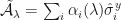$\Tilde{\mathcal{A}}_{\lambda} = \sum_i \alpha_i(\lambda) \hat{\sigma}_i^y$ into the equation I mentioned above, you can use a variational procedure to find exactly what the coefficients $\alpha_i(\lambda)$ should be! Putting it another way: once you pick some truncated version of the CD, you’ll know exactly how it contributes to the full thing. The coefficients $\alpha_i(\lambda)$ turn out to be, as one would expect, functions of the terms in the Hamiltonian.

This approximate CD can be as simple to engineer as you’d like it to be, since you have completely free choice of operators. If the operators are not part of the AGP, the variational procedure will simply tell you that their coeffcients are 0. And it does the most wonderful thing: it lets you drive your system faster than you ever could without it, with the same amount of losses/transitions! Its job is to suppress most of them, even if it can’t suppress all.

To end on an example, I’ll show you what happens when your ansatz is exact. Take a Hamiltonian for a single spin which starts in its ground state, with a time-dependent angle $\phi(t) = \pi \frac{t}{\tau}$ that evolves for total time $\tau$ :

$H(t) = -h \begin{pmatrix} \cos{\theta} & e^{i \phi(t)}\sin{\theta}\\ e^{-i \phi(t)}\sin{\theta} & \cos{\theta} \end{pmatrix}$ .

Since we’re only working with a single spin, we’d imagine that all its degrees of freedom are captured by a combination of single-spin operators. In fact, the full CD drive in this case is made up of just $\sigma^z$ , with a coefficient drive we can find variationally to just be: $\alpha(t) = \frac{\pi}{2 \tau}$ . The counterdiabatic Hamiltonian which suppresses all transitions is then:

$H_{\rm CD}(t) = H(t) + \alpha(t)\sigma^z$ .

We can visualise how the evolving spin follows the ground state of the instantaneous Hamiltonian $H(t)$ exactly throughout the evolution in the animation below:

Animation of the Hamiltonian’s real and imaginary parts for non-adiabatic and CD evolution, as well as the evolving state of the system on the corresponding Bloch spheres. The total evolution time is $\tau = \pi$ . Here, $\theta = \frac{\pi}{4}$ .

Animation of the Hamiltonian’s real and imaginary parts for non-adiabatic and CD evolution, as well as the evolving state of the system on the corresponding Bloch spheres. The total evolution time is $\tau = \pi$ . Here, $\theta = \frac{\pi}{4}$ .

COLD

Finally, after all the groundwork is set, we can get to the main course: Counterdiabatic Optimal Local Driving. While it may seem like I spent an awful lot of time on related topics to get here, it’s near impossible to explain COLD without a decent understanding of the variational approach/LCD. COLD is a product of wanting to explore the shortcomings of LCD and to improve upon them. This is what we set out to do and this is what (I’m happy to report) we achieved!

First off, a key reason to try and improve on the LCD is that it is generally an approximate approach. Unless your ansatz contains all the necessary operators (which for anything worth your time, it probably won’t), you’ll only ever get a truncated CD out of the procedure. This means that there are cases where it might perform abysmally at suppressing losses from non-adiabatic effects.

The second thing to note is that the efficiency of a particular choice of ansatz is related to the path your Hamiltonian takes in time. What I mean by this is that you can choose any time-dependent functions to vary your Hamiltonian from its initial to its final form. For the pure adiabatic protocol, all that matters is that the starting/ending points are the same, since these should have the required ground states. In our animation example, my variable $\phi(t)$ could have taken any path from the value of 0 to $\pi$ . In fact, I could have varied $\theta$ in time too, and it would not have mattered as long as it started at and returned to the same value in the beginning and end of the protocol, given you were driving infinitely slowly,

However, the path really does matter for anything that happens in finite time. It matters specifically because it determines the form of the AGP. I didn’t make this explicit, but it drops straight out of the variational approach when you try it out.

The path taken by the Hamiltonian in parameter space doesn’t matter in principle as long as the start/end points are the same – the ground states of the initial and final Hamiltonians stay the same. The non-adiabatic effects, however, are highly dependent on the path taken and hence the CD is determined by the way the Hamiltonian evolves in time.

Okay, so what do we do with this information? Our goal, as with any counterdiabatic protocol, is to drive a time-dependent Hamiltonian as quickly as possible with as few losses/transitions out of the eigenstate as possible. We have several problems:

We can’t derive the perfect CD.
We have a time limit on how fast we want to drive our system because at longer times decoherence becomes a big problem. Unfortunately, this time limit leads to huge non-adiabatic effects that make our protocol near-useless.
Even if we could derive the perfect CD, there would be no way to engineer most of the operators required – we’re mostly confined to highly local things like $\sigma^y$ .
The best option we have, the variational approach, seems to give a pretty bad suppression of losses for the operators we can engineer.

That all sounds pretty bad what can a poor experimental physicist do? Well, luckily, they can implement a brand new method called COLD, of course!

COLD, illustrated: a generally slow-moving turtle being shuttled through the air at insane speeds with a jetpack strapped to its back! Who said we couldn’t do adiabatic protocols quickly? (credit to DALL-E 2)

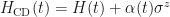
COLD takes the variational approach and the idea that it depends on the path of the Hamiltonian and does the obvious next step: engineering a new path, one with the same initial and final Hamiltonian, but with a much more favorable form of the AGP.

We’re happy to take your constraints into account: local operators, limits on power and obviously, the problem Hamiltonian. What we’ll add onto the variational approach is controllability: say you have the ability to engineer different Hamiltonians with the same start and end points. Given all possible paths you could take, we propose optimising for the path that maximises how well your ansatz LCD deals with the non-adiabatic effects.

This idea comes from control theory, and the field of quantum optimal control, by no means a novel idea. What we propose to do is to either engineer the path of a given degree of freedom (like the angle $\phi(t)$ in our earlier example) or to add new degrees of freedom that are easy to manipulate and control, like an extra set of operators. You might ask how different this is to choosing an ansatz for the AGP and the answer is simple: the AGP is pre-determined for a given Hamiltonian. The variational approach only tells you the best you can do with what you’ve got. What we propose is to add controllable drives that are not part of the AGP in order to make the job of the CD easier.

An example of two possible paths, in 3D parameter space $(\phi, \theta, \beta)$ : one follows an arbitrary path which leads to large losses due to non-adiabatic effects (symbolised by the large norm of the AGP). The other minimizes these losses by playing to the strengths of an approximate CD with a given ansatz set of operators and minimizing the norm of the AGP throughout the evolution.

An example of two possible paths, in 3D parameter space $(\phi, \theta, \beta)$ : one follows an arbitrary path which leads to large losses due to non-adiabatic effects (symbolised by the large norm of the AGP). The other minimizes these losses by playing to the strengths of an approximate CD with a given ansatz set of operators and minimizing the norm of the AGP throughout the evolution.

Picture COLD as including an extra step in the process of the LCD: we take our original Hamiltonian $H(\lambda)$ and add a control drive with optimisable parameters $\beta_j(\lambda) \in \boldsymbol \beta$ to it with some easily engineered set of operators $\hat{O}_j$ that aren’t part of the AGP:

$H(\lambda, \boldsymbol \beta) = H(\lambda) + \sum_j \beta_j (\lambda) \hat{O}_j$

Then, include an LCD drive with some limited set of operators that combat the non-adiabatic effects:

$H_{\rm COLD}(\lambda, \boldsymbol \beta) = H(\lambda, \boldsymbol \beta) + \alpha(\lambda, \boldsymbol \beta)\hat{O}_{\rm LCD}$ .

Notice how the $\alpha$ ‘s depend on the optimisable coefficients $\boldsymbol \beta$ ? This is because the new control drive is there to change the path of the Hamiltonian. In our above illustration, it’s like adding a new dimension in which the path can exist. Since the AGP and the non-adiabatic effects are determined by the Hamiltonian’s path, changing the parameters $\beta_j (\lambda)$ changes the CD for the system. In fact, it can change it in a way that makes it maximally effective for the choice of ansatz parameters.

All that remains is to pick the right type of control drive and to optimise the parameters. We could do this with several different targets in mind, though the usual one is the final fidelity of the Hamiltonian’s final ground state. This is stuff I won’t get into in detail because this blogpost is already far too long and if you’ve read up to this point and want to know more then I’d recommend reading our paper on arXiv or on PRX Quantum 🙂 However I will leave you with a quick animation that shows how these things perform on a simple example:

Example showing a two-spin annealing process which you can find in our paper. I’m plotting only one of the spins’ Bloch spheres for clarity here. The top line is just $H(\lambda)$ , the middle is the LCD approach with $\sigma^y$ operators as ansatz and the final line includes an optimisable drive (ie COLD). We can check how the final fidelities fare for each and though it’s a simple, easy model, COLD still has space to improve on the LCD.

Example showing a two-spin annealing process which you can find in our paper. I’m plotting only one of the spins’ Bloch spheres for clarity here. The top line is just $H(\lambda)$ , the middle is the LCD approach with $\sigma^y$ operators as ansatz and the final line includes an optimisable drive (ie COLD). We can check how the final fidelities fare for each and though it’s a simple, easy model, COLD still has space to improve on the LCD.

Final notes

So here it is, a relatively brief introduction to a piece of work that took us a year and a half to explore and put together. There is a lot more I want to say, eg how much there is left to explore and some of the insane insights we got while working on this (hint: the AGP contains a LOT of information about your system, more than you can see on the surface).

Instead, I’ll leave you with an invitation to read our work, reach out to me with further questions (I’ll be delighted to engage), read some of these [1], [2], [3] for more cool insights into the AGP and most of all to let me know if I should cover anything else surrounding this topic and if so, what.

Thank you for reading.

Adiabatic quantum computation

A slightly deeper dive into CD

The variational approach

COLD

Final notes

Share this:

Like this:

Leave a Reply Cancel reply