Fusion-based Quantum Computing 1: Building Blocks

In January of 2021, a bunch of people from Palo-Alto-based quantum startup PsiQuantum posted a paper on the arXiv introducing “fusion-based quantum computation” (FBQC), a brand new quantum computing paradigm and a variant of measurement-based quantum computation (MBQC). This is exciting for several reasons: the scheme is a contender for scalable, fault-tolerant quantum computation and it offers several interesting advantages over the usual circuit-based quantum computing (CBQC) model as well as MBQC.

Since the original paper several more (1, 2, 3) made their appearance on the arXiv, refining the initial ideas and offering an insight into the details of an actual implementation of the scheme on a photonics-based hardware set-up (more on that later). Given these developments, there now appears to be enough information to properly understand and (optimistically) envision a world where FBQC is a mainstream approach to performing quantum computation. While I am by no means trying to endorse FBQC, I find it pretty interesting and credible as a future quantum computing paradigm. This is the main reason for starting a series of blog posts – the first of which you’re reading now.

I was lucky enough to get the chance to delve into PsiQuantum’s entire body of work on FBQC during my 3-month internship at a Cambridge-based quantum startup Riverlane (wonderful experience – might write about that sometime in the future). The concept of FBQC is pretty recent and I haven’t found too much about it out there on the internet yet (except for this small excited mention on Scott Aaronson’s blog) so given my inundation in the subject and love for science communication, it only feels right to put something together and put it out there so that the quantum community might make use of it.

This first post concerns itself only with the basics of FBQC, the so-called primitives for computation: fusion, resource states and a brief glimpse at fusion networks. Most of the information required to understand it is in the original FBQC paper and the one thing I’d recommend really reading up on is basic quantum error correction (QEC) and stabilizers/groups. I’ll try to motivate and explain things as I go but the assumption going into this is that the reader will have a decent understanding of the basics of quantum mechanics/computing and of the stabilizer formalism.

Before I start, a small disclaimer: I hadn’t really delved too much into fault-tolerance or linear optics (photonics) quantum computing before landing the internship so my expertise on these subjects is limited. FBQC itself is something I learned about only in the last few months and it’s very likely that I say something slightly wrong or misrepresent some part of it, so criticism and feedback are always very welcome.

Fusion and the One-Way Computer

So what is FBQC? This is a question that requires several blog posts to answer in full in my case, but before I start on the details I’ll attempt to give some intuition. The main idea behind FBQC is that information is transmitted and processed through teleportation, same as in MBQC model (and very differently from the static, circuit-based approach that most of us are used to). This teleportation happens between small entangled resource states and is mediated via fusion measurements, which are like the sewing thread stitching together a giant fabric of correlations between the qubits. This teleportation-style computation is also why the most natural context for actually implementing FBQC is photonics/linear optics, where photons reign supreme and measurements are destructive (your qubits don’t really stick around after they hit the detector).

So what’s a fusion (measurement) then? In the context of photonics they are a way to achieve entanglement – although only between already-entangled states (it’s not complicated, I’ll explain in a bit). Photons don’t interact much so they don’t really suffer from decoherence, but this also means they don’t get entangled very easily making this is a pretty key operation for any photonics system that wants to do a useful quantum computation. The long and short of it all is that fusions in FBQC are two-photon destructive measurements which are inherently probabilistic i.e. they have some (detectable) probability of failure.

Quick aside to let you know that I won’t go into any of the math behind fusion here because I want to make this more of an overview of the process than an in-depth tutorial, but I’m happy to do that in a different post if this is something people find interesting.

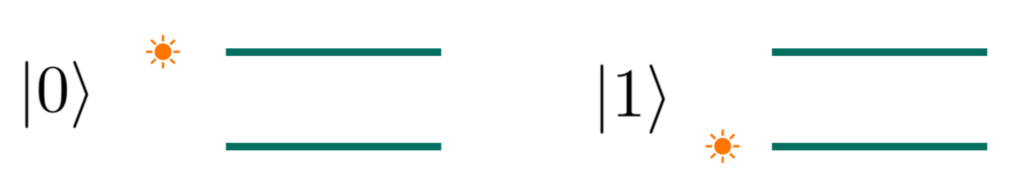
In PsiQuantum’s set-up which uses dual-rail encoding for their qubits (see picture below), both photons have to be measured – this is known as Type-II fusion. Whether or not the fusion is a success can be checked if both detectors used in the measurement emit a ‘click’ (a lack of click would, for example, mean that the photon got lost somewhere in the process by interacting with the environment).

Dual-rail encoding of qubits, where a single photon (lil’ sun) is present in one of two waveguides (spatial modes/degrees of freedom, thick green lines) representing the two computational basis states (|0> and |1>). Note that in this set-up there is an additional degree of freedom in the polarisation of the photon which isn’t really visible but plays a part in the whole thing.

In the case of a successful fusion, you get two measurement outcomes, depending on which basis you measure in. The FBQC literature tends to focus is generally on joint outcomes $\langle XX, ZZ \rangle$ or $\langle XZ, ZX \rangle$ (in a different basis) where $XX$ for example stands for $X \otimes X$ on the two photons involved. The parities (±1) of these outcomes tells you which exact state your leftover qubits end up in.

Ah, yes, I’ve sort of kept this part a tad quiet so far: in the contexts of MBQC (where fusions are used to create large cluster states) and FBQC alike, larger entanglement can only be created from smaller entanglement. So you start with something like Bell pairs (which can be generated without fusion) and then build up a larger correlated/entangled cluster by fusing parts of them together. Note, Type-I fusion only measures one photon so you can just keep adding to this cluster until it’s big enough.

This makes sense when you consider that fusions are destructive measurements. What actually happens in FBQC is that we take two so-called resource states which already have some amount of entanglement present and we perform fusion between them. This propagates entanglement correlations through the unfused system – the qubits/photons that were entangled with those that are lost in the fusion maintain the information .

Here’s a simple example (which I’ll explore in more detail and with more help from the stabilizer formalism + animations further down in the post): say I have two maximally entangled states A and B, perhaps two Bell pairs. Note that at this point A and B share no entanglement between them, only within each system. We can label the qubits A1 and A2 in resource state A and B3, B4 in resource state B.

Say I now perform a fusion measurement between A2 and B3 and in the process I destroy both. Well, now all I have left is a new quantum state C made of qubits A1 and B4 as well as two classical bits of information – the joint measurement outcomes of A2 and B3. The interesting thing is that by performing the fusion successfully, I leave the qubits A1 and B4 entangled with each other, their new state C described in part by the outcomes of the measurement on A1 and B1. I’ve essentially propagated information from $A \otimes B$ to $C$ by destroying parts of A and B but joining the leftovers! This gets a lot more interesting when A and B are made up of more than two qubits.

Figure from the original FBQC paper featuring an example of three resource states: (1,2,3), (4,5) and (6,7,8) where indices label qubits and brackets separate the individual resource states. It shows two separate fusions in the <XZ, ZX> basis (the Ms here are the ±1 outcomes of the measurements) on qubits <3,4> and <5,6> which result in a final entangled state made up of qubits (1,2,7,8).

Computational lego blocks: resource states

Given I’ve mentioned resource states more than enough times already, I figured it might be a good idea to discuss what they actually are in the context of FBQC. Before we do that though, I’ll mention a thing or two about the stabilizer formalism, which is something I once again recommend being familiar with if you want to delve deeper into FBQC and quantum error correction in general.

In the stabilizer formalism, you describe your quantum states by what operations leave them invariant. i.e. stabilize them. A stabilizer state on n qubits is a state that is a +1 eigenstate of a size 2ⁿ subgroup of Pauli operators. The nicest example of this is always the Bell pair state 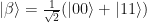$|\beta\rangle = \frac{1}{\sqrt{2}} (|00\rangle + |11\rangle)$ , where for 2 qubits we have the set of 4 operators $\{II, XX, YY, ZZ \}$ which leave it unchanged. You can test this out by checking that, e.g. $XX|\beta\rangle = |\beta\rangle$ .

This is a really nice language to talk about quantum states since it a) saves you the trouble of writing out complex vectors and density matrices (the set of stabilizing operators is enough to tell you exactly what state you’re talking about) and b) helps you track what happens to states after some measurement of the system or its subsystems is made. A measurement in some basis changes the stabilizers according to a pretty simple set of rules so even if you make many measurements and have to keep track of many outcomes, you have a very nice way to keep track of what your state IS at any point in the computation. Furthermore, you don’t even need to write out all of the 2ⁿ stabilizers, you can simply work with a small subset called the generators.

(By the way if you want to know more about this stuff and if you’ve not yet done so, I recommend reading the Quantum Bible – “Quantum Computation and Quantum Information” by Nielsen and Chuang – starting from around page 454. They do a great job of explaining everything super concisely.)

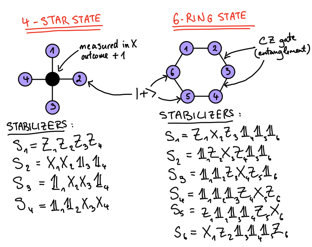
The reason I bring this up is because that’s exactly how we’ll talk about resource states in FBQC. Resource states are small and that comes from the difficulty of generating large entangled states on demand. In the original FBQC paper we get two examples: 4-qubit “star” states and 6-qubit “ring” states. The latter is one that we’ll come back to in future posts so I’ll focus on it a bit more.

I should mention that in principle you can use different types of resource states – these are just ones which have already been shown to be useful in building up large-scale computations. In fact, the whole idea of choosing a good resource state comes down to whether or not you can exploit its symmetries to come up with a fault-tolerant, topological quantum computing scheme. These are things I’ll come back to in future posts but it’s something I wanted to bookmark just now.

Graph states

To understand both the 4-star and the 6-ring states, we need one last piece of the puzzle and this is one that is very familiar to anyone that’s ever worked with MBQC: graph states. The basic idea is that you have a simple way to generate and describe the large entangled cluster states needed for an MBQC computation, specifically via stabilizers. Luckily, the graph state formalism turns out to be useful in FBQC too.

Take your qubits to be vertices on a graph and have them all be initialized in the $|+\rangle$ state. Then, entangle them using $CZ$ (controlled-Z) operations according to the edges on this graph. The graph itself is just an abstract construction that defines your computation so you know how many qubits you need and which of them need to be entangled with which other qubits accordingly. In MBQC these large cluster states come from graphs of cubic lattices while in FBQC they are used to describe your resource states. I’ll give a preview below for both the 4-star and the 6-ring so you get the idea:

Illustration of the 4-star and 6-ring resource states along with their stabilizer generators. The qubits are the vertices (purple circles) and they’re entangled with CZ gates according to the edges. Note the black centre in the 4-star – I’ll talk about that in a second.

One of the main reasons for using this graph paradigm is that (you guessed it) the stabilizers for these things are well-understood and easy to work with. The algorithm is this: for each qubit i in the graph, you’ll have a stabilizer of the form

$S = X_i \prod_{j \in \mathcal{N}_i} Z_j$ ,

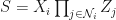
where $\mathcal{N}_i$ are the neighbours (i.e. connected by an entangling edge) of the i^th qubit. You can see that nicely in the picture above in the 6-ring case, where for the six qubits you have six stabilizers of the form $Z_{n-1} X_n Z_{n+1}$ (with indices wrapping around) since each has two neighbours and hence two Z operators.

What about the 4-star state, you might ask? Well this one is interesting because it still exploits the graph state formalism but with a twist. What you do is you start with a 5 qubit graph state as in the picture and then you measure the central one in the X-basis. Conditioned on the outcome being +1, what you’re left with is a different sort of entangled state: a GHZ state. You can see that the form of the stabilizers for this is also different. I won’t really focus on the 4-star so I won’t go into too much detail but it works as a nice example to have as an alternative to the 6-ring.

Putting it all together

Okay, so we’ve got resource states and we know that we fuse together these things using fusion measurements and that this propagates entanglement and correlations. This is all well and good but what we really want to do is to compute something using these components and operations. Not only that – we want to have some sort of redundancy involved so that we could perform error correction and get fault-tolerance out of it. AND we want to be able to scale these things up and understand/control what’s happening to the information propagating throughout the computation regardless of how complex it is.

I’ll briefly address the “compute” part in this post, just to whet the appetite. Sadly, you’ll have to wait for the large-scale error correcting fusion network main course until the next post (and then perhaps some delicious fault-tolerant channels for dessert in an even later post – I’ve taken this metaphor a little too far now).

So what does it mean to compute in this setting? Generally you’d picture some input information encoded in a quantum state, followed by some sort of processing (unitary evolution, measurements etc.), followed by an output state or classical set of measurement outcomes. In the circuit model this is pretty simple – you picture your input as qubits (lines/complex vectors) initialised in some state, processing as unitaries/gates (boxes/operators) and your output can be either the changed/processed quantum state (still lines/complex vectors) or classical information (measurement outcomes, strings of 1s and 0s).

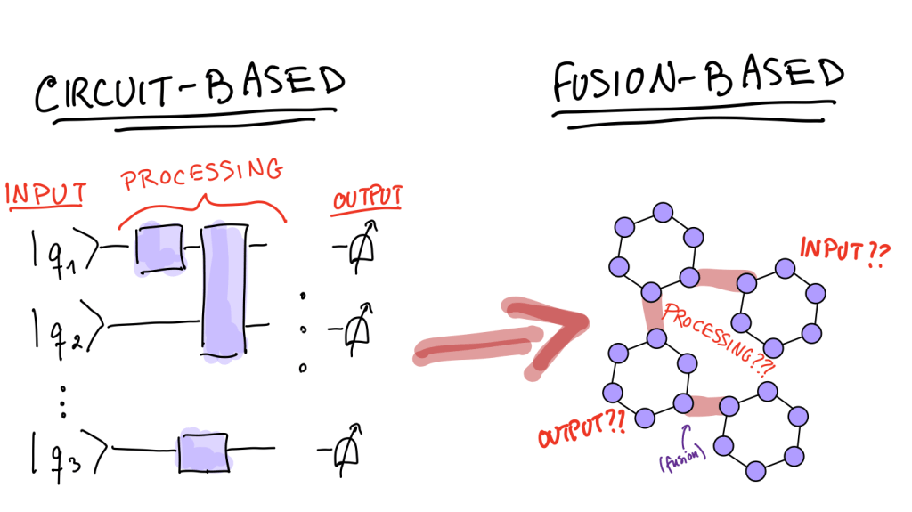
In FBQC the structure on a larger scale isn’t quite as simple, but the basic notions of input, processing and output can be captured very nicely with groups and stabilizers. Instead of complex vectors, the input is a stabilizer group R which describes the resource states – e.g. for one 4-star state we would have $R = \langle ZZZZ, XXII, IXXI, IIXX \rangle$ (where I omitted the qubit indices). Instead of unitaries, for processing we have something called a fusion group F (which is not a stabilizer group!) that contains the fusion measurements which you want to perform as well as a $-I$ for convention (its purpose will become more obvious, don’t worry). So if you want to perform a single fusion in the XX/ZZ basis between some two qubits as your computation, you’d have $F = \langle XX, ZZ, -I\rangle$ .

Finally, your output should be either another quantum state (to e.g. act as input for the next computation) or classical outcomes. The latter is easy to picture: you already have your joint measurement outcomes from the fusions and you could simply do single-qubit measurements on the leftover state post-fusion to get a bunch of classical data out. In the former case however, it only makes sense to end up with another stabilizer group, which we’ll refer to as the surviving stabilizer group S. This should contain the set of elements (not generators!) of R that commute with all elements of F on account of the fact that if a measurement doesn’t commute with all stabilizers of a state then the stabilizers have to be updated accordingly.

But wait! There’s more! S might still contain operators of qubits/photons that got destroyed in the fusion (i.e. 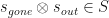$s_{gone} \otimes s_{out} \in S$ where $s_{gone}$ are the destroyed qubits and $s_{out}$ are those leftover, acting as output). What we actually want to end up with are stabilizers for the unfused qubits and informed by the set of measurement outcomes of the fusions. If, say, a measurement outcome of the fusion is $m^{XX} = \pm 1$ , we can see it as projecting into a space $m^{XX}XX \in s_{gone}$ and then instantly being destroyed. So instead we take $m s_{gone} \otimes s_{out} \rightarrow m s_{out} \in S_{out}$ . This $\boldsymbol{S_{out}}$ is the output stabilizer group which actually gives us the output state we were after!

How does all of this look in pratice?

I’ll illustrate the above way of looking at computation with an example which will be a nice way to put everything together. Let’s go back to the simple two Bell-pair example we had before but spice it up a little by choosing to use graph states instead. Remember this means we take two qubits in the $|+\rangle$ state and entangle them with a CZ operation, ending up with something like: $|\psi\rangle = \frac{1}{2}(|00\rangle + |01\rangle + |10\rangle - |11\rangle)$ . We know then, that the first pair of these can be described with the stabilizers $X_1Z_2$ and $X_2Z_1$ (feel free to check this) while the second pair mirrors with $X_3Z_4$ and $X_4Z_3$ . So we have:

$R = \langle (X_1Z_2, X_2Z_1), (X_3Z_4, X_4Z_3)\rangle$

Where the curved brackets are there just to differentiate between the two resource states. We fuse qubits 2 and 3 so take $F = \langle X_2X_3, Z_2Z_3, -I\rangle$ . This will give two measurement outcomes, $m^{XX}, m^{ZZ} \in \{-1, +1\}$ .

Bear in mind that to get S we need to multiply together elements of R since they anticommute with those in F. Doing that gives us $S = \langle X_1Z_2Z_3X_4, Z_1X_2X_3Z_4 \rangle$ and we simply replace the operators for qubits 2 and 3 with the measurement outcomes giving:

$S_{out} = \langle m^{ZZ}X_1X_4, m^{XX}Z_1Z_4\rangle$

I’ve made a short animation to illustrate this process, where you can see that the leftover state is made up of qubits 1 and 4 (which, if you noticed in S_out, are now Bell pairs instead of graph states!).

Conclusion and hyping of next part

So there we are: a brief introduction to the FBQC paradigm. There’s a lot left to address, including how to perform universal operations/gates as well as error-correction and large-scale computation. These are things I plan to talk about in the next blog post or two, which will hopefully take less than forever to put out.

Finally, I really recommend watching this tutorial by Naomi Nickerson – one of the authors of FBQC – in order to get an intuition both for fault-tolerance and FBQC. It’s long but very engaging and an absolute treasure for getting into the whole thing.

I hope this was interesting and useful and would love to have feedback!